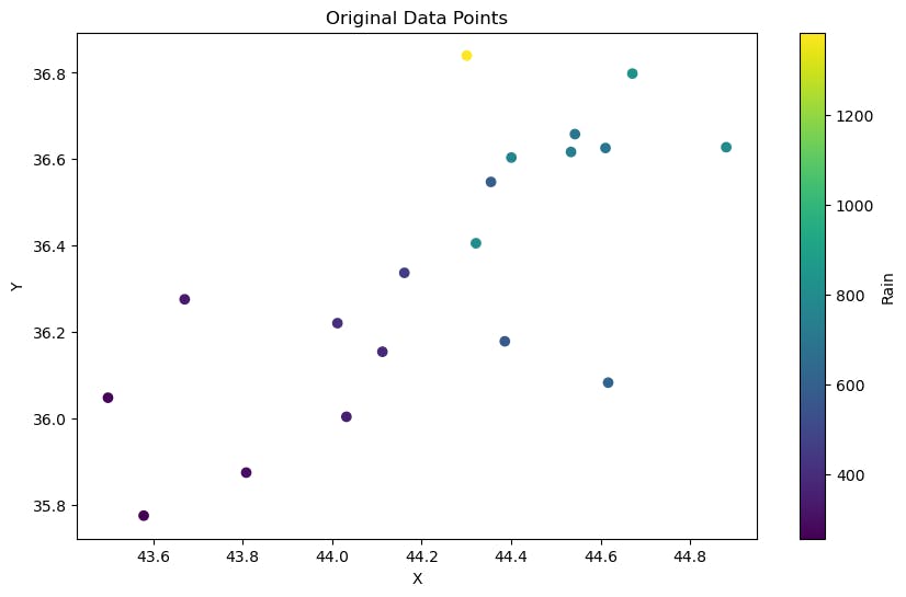
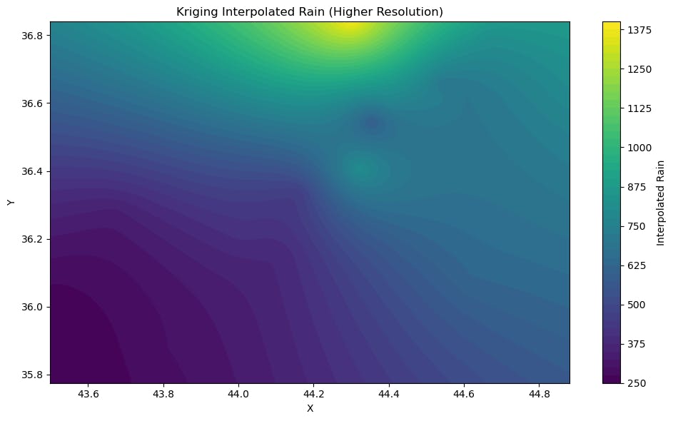
This code performs spatial interpolation of rain data using kriging, enabling the estimation of rain values at unmeasured locations within the Erbil Governorate, based on the available data.
1. Importing Necessary Libraries:
pandas: Used for loading and manipulating tabular data, like the CSV file.
numpy: Provides efficient array operations for numerical computations.
pykrige.ok: Offers the OrdinaryKriging class for performing kriging interpolation.
matplotlib.pyplot: Used to visualize data and create plots.
2. Loading Data:
data =pd.read_csv("Erbil_Rain.csv"): Reads rain data from a CSV file named "Erbil_Rain.csv" into a pandas DataFrame.
| station | rain | x | y |
| Qushtapa | 350 | 44.0319 | 36.0039 |
| Ainkwawa | 414 | 44.0119 | 36.2206 |
| Khabat | 339 | 43.67039 | 36.2758 |
| Bnaslawa | 381 | 44.1124 | 36.15444 |
| Shorsh | 566 | 44.386 | 36.1786 |
| Shaqlawa | 810 | 44.3214 | 36.4056 |
| Harir | 591 | 44.355 | 36.5475 |
| Khalifan | 768 | 44.4006 | 36.6039 |
| Soran | 701 | 44.5428 | 36.6581 |
| Rwandz | 736 | 44.5339 | 36.6169 |
| Choman | 796 | 44.8808 | 36.6278 |
| Sidakan | 824 | 44.6711 | 36.7983 |
| Mergasor | 1384 | 44.3008 | 36.84 |
| Makhmwr | 257 | 43.57887 | 35.77511 |
| Bastora | 457 | 44.16148 | 36.33709 |
| Dibaga | 299 | 43.808 | 35.8747 |
| Gwer | 269 | 43.499 | 36.048 |
| Barzewa | 700 | 44.611 | 36.626 |
| Koya | 622 | 44.617 | 36.083 |
3. Extracting Data:
x = data['x']y = data['y']rain = data['rain']: Extracts the x-coordinates, y-coordinates, and rain values from the DataFrame.
4. Creating a Kriging Object:
ok = OrdinaryKriging(x, y, rain, variogram_model='linear', verbose=False): Creates an instance of OrdinaryKriging for spatial interpolation, using a linear variogram model.
5. Defining a Grid for Interpolation:
grid_x = np.linspace(min(x), max(x), 100)grid_y = np.linspace(min(y), max(y), 100): Creates evenly spaced grid points in the x and y directions, covering the spatial extent of the data.
6. Performing Kriging Interpolation:
z, ss = ok.execute('grid', grid_x, grid_y): Performs kriging interpolation on the defined grid, estimating rain values at each grid point and providing associated kriging variance (or squared standard deviation).
7. Plotting Original Data Points:
plt.scatter(x, y, c=rain, cmap='viridis', label='Original Data'): Creates a scatter plot of the original data points, with colors representing rain values.
8. Plotting Interpolated Surface:
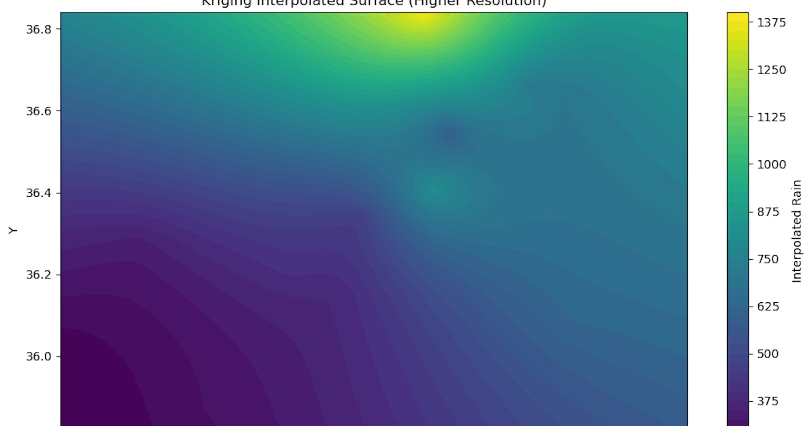
plt.contourf(grid_x, grid_y, z, cmap='viridis', levels=50): Creates a contour plot of the interpolated rain surface, smoothly visualizing the predicted rain values across the entire grid.
9. Displaying Plots:
plt.show(): Shows both plots to visualize the original data and the interpolated surface.


The full code is presented below:
import pandas as pd
import numpy as np
from pykrige.ok import OrdinaryKriging
import matplotlib.pyplot as plt

# Load data from CSV
data = pd.read_csv("Erbil_Rain.csv")

# Assuming the columns are named station, rain, x, and y
x = data['x']
y = data['y']
rain = data['rain']

# Create an instance of OrdinaryKriging
ok = OrdinaryKriging(x, y, rain, variogram_model='linear', verbose=False)

# Define a grid to interpolate
grid_x = np.linspace(min(x), max(x), 100)  # Adjust the number of points as needed
grid_y = np.linspace(min(y), max(y), 100)  # Adjust the number of points as needed

# Perform kriging interpolation on the defined grid
z, ss = ok.execute('grid', grid_x, grid_y)

# Plotting original data points
plt.figure(figsize=(10, 6))

# Plot original data points
plt.scatter(x, y, c=rain, cmap='viridis', label='Original Data')
plt.colorbar(label='Rain (mm)')
plt.title('Original Data Points')
plt.xlabel('X')
plt.ylabel('Y')

# Contour plot of the interpolated surface
plt.figure(figsize=(10, 6))
plt.contourf(grid_x, grid_y, z, cmap='viridis', levels=50)
plt.colorbar(label='Interpolated rain (mm)')
plt.title('Kriging Interpolated Rain')
plt.xlabel('X')
plt.ylabel('Y')

plt.tight_layout()
plt.show()
