In this tutorial, you learn how to perform in Python descriptive statistics (i.e min and max), central tendency (i.e. mean and median), variability (i.e. variance and standard deviation), summary, correlation (i.e. covariance and correlation coefficient), and statistical tests (i.e. t-test). We use statistical powerful libraries such as scipy.stats function in SciPy library, scikit-learn, statsmodels, and other libraries.
Import libraries:
import numpy as np
import pandas as pd
import statistics
import scipy.stats
from statsmodels.formula.api import ols
from scipy import stats
Descriptive statistics
x = [11, 13, 8, 16, 23, 24, 30, 16, 9, 18] # create a list
x = np.array(x) # convert x to numpy array
Min
print(x.min())
# 8
Max
print(x.max())
# 30
Mean
print(x.mean())
# 16.8
Var
print(x.var())
# 45.36
Sum
print(x.sum())
# 168
Median
print(np.median(x))
# 16
Measures of central tendency:
To measure the central or middle values of datasets we can use: mean, weighted mean, geometric mean, harmonic mean, median, mode.
Mean
print(x.mean())
# 16.8
# or
mean = sum(x) / len(x)
mean
# 16.8
Harmonic mean
hmean = len(x) / sum(1 / item for item in x)
hmean
# 14.225214542387663
Weighted mean
y = [1, 3, 5, 7, 9, 10, 12, 14, 15, 16]
wmean = sum(y[i] * x[i] for i in range(len(x))) / sum(y)
wmean
# 18.0
Geometric mean
scipy.stats.gmean(x)
# 15.47120474800591
Median
statistics.median(x)
# 16.0
Mode
statistics.mode(x)
# 16
Measures of variability
It calculates the spread of data points such as variance, standard deviation, skewness, percentiles, ranges.
Variance
statistics.variance(x)
# 50
Standard deviation
statistics.stdev(x)
# 11.099549540409287
Skewness
scipy.stats.skew(x, bias=False)
# 0.5846768190780606
Percentiles
np.percentile(x, 5) # the 5th percentile
# 8.45
np.percentile(x, 95) # the 95th percentile
# 27.299999999999994
np.percentile(x, [25, 50, 75]) #25th, 50th and 75th percentile
# array([11.5 , 16.  , 21.75])
Range (maximum - minimum)
np.ptp(x)
# 22
max(x)-min(x)
# 22
Summary of descriptive statistics
scipy.stats.describe(x, bias=False) # correcting the skewness and kurtosis for statistical bias
# DescribeResult(nobs=10, minmax=(8, 30), mean=16.8, variance=50.400000000000006, skewness=0.5846768190780606, kurtosis=-0.42418400340735873)

x = pd.Series([22, 13, 14, 55, 10])
x.describe() # Using pandas function
"""
count     5.000000
mean     22.800000
std      18.539148
min      10.000000
25%      13.000000
50%      14.000000
75%      22.000000
max      55.000000
dtype: float64
"""
Measures of correlation
(Tip: Correlation implies association, not causation.)
Correlation coefficient and covariance can measure the correlation between variables.
Covariance
# create x and y list
x = [11, 13, 8, 16, 23, 24, 30, 16, 9, 18]
y = [1, 3, 5, 7, 9, 10, 12, 14, 15, 16]

cov_matrix = np.cov(x, y)
cov_matrix
cov_xy = cov_matrix[0, 1] # or [1, 0]
cov_xy
# 12.266666666666667
Correlation coefficient
Pearson correlation coefficient (r) is a measurement of the correlation between data.
r, p = scipy.stats.pearsonr(x, y) # using pearsonr stats function of SciPy library
r
# 0.3348799480266361
corr_matrix = np.corrcoef(x, y) # using corrcoef from NumPy
corr_matrix
r = corr_matrix[0, 1]
r
# 0.33487994802663607

lg = scipy.stats.linregress(x, y) # extract r from linregress of SciPy library.
# LinregressResult(slope=0.24338624338624337, intercept=5.111111111111111, rvalue=0.33487994802663607, pvalue=0.3442215013372624, stderr=0.24212131035281)
r = lg.rvalue
r
# 0.33487994802663607
We can calculate it from the formula:
std_x=statistics.stdev(x)
std_y=statistics.stdev(y)
cov_xy = 12.26666666666
r = cov_xy / (std_x * std_y)
r
# 0.33487994802645404
Student’s t-test
stats.ttest_1samp(x, 0)   # one sample
# Ttest_1sampResult(statistic=7.483314773547883, pvalue=3.75801166724644e-05)
stats.ttest_ind(x, y)   # two sample
#Ttest_indResult(statistic=2.738454755684762, pvalue=0.01350066550703028)
Ordinary least squares (OLS)
df = pd.DataFrame({'x': x, 'y': y}) # create data frame

model = ols("x ~ y + 1", df).fit()
print(model.summary())

"""
 OLS Regression Results
=========================================================================
Dep. Variable:                      x   R-squared:                       0.112
Model:                            OLS   Adj. R-squared:                  0.001
Method:                 Least Squares   F-statistic:                     1.010
Date:                Sun, 04 Jul 2021   Prob (F-statistic):              0.344
Time:                        06:07:07   Log-Likelihood:                -32.668
No. Observations:                  10   AIC:                             69.34
Df Residuals:                       8   BIC:                             69.94
Df Model:                           1
Covariance Type:            nonrobust
=========================================================================
                 coef    std err          t      P>|t|      [0.025      0.975]
------------------------------------------------------------------------------
Intercept     12.5609      4.777      2.630      0.030       1.546      23.576
y              0.4608      0.458      1.005      0.344      -0.596       1.518
=========================================================================
Omnibus:                        0.271   Durbin-Watson:                   1.243
Prob(Omnibus):                  0.873   Jarque-Bera (JB):                0.313
Skew:                           0.290   Prob(JB):                        0.855
Kurtosis:                       2.357   Cond. No.                         22.3
=========================================================================

Warnings:
[1] Standard Errors assume that the covariance matrix of the errors is correctly specified.
"""
Multiple Regression (multiple factors)
x = [11, 13, 8, 16, 23, 24, 30, 16, 9, 18]
y = [1, 3, 5, 7, 9, 10, 12, 14, 15, 16]
z = [2, 4, 6, 8, 10, 11, 13, 15, 17, 19]
df = pd.DataFrame({'x': x, 'y': y, 'z':z})
model = ols('x ~ y + z', df).fit()
print(model.summary())

"""
 OLS Regression Results
=========================================================================Dep. Variable:                      x   R-squared:                       0.291
Model:                            OLS   Adj. R-squared:                  0.089
Method:                 Least Squares   F-statistic:                     1.439
Date:                Sun, 04 Jul 2021   Prob (F-statistic):              0.300
Time:                        06:23:49   Log-Likelihood:                -31.541
No. Observations:                  10   AIC:                             69.08
Df Residuals:                       7   BIC:                             69.99
Df Model:                           2
Covariance Type:            nonrobust
=========================================================================
                 coef    std err          t      P>|t|      [0.025      0.975]
------------------------------------------------------------------------------
Intercept     15.7079      5.139      3.057      0.018       3.556      27.859
y              6.5891      4.627      1.424      0.197      -4.351      17.530
z             -5.6693      4.261     -1.331      0.225     -15.745       4.406
=========================================================================
Omnibus:                        0.842   Durbin-Watson:                   1.785
Prob(Omnibus):                  0.656   Jarque-Bera (JB):                0.626
Skew:                          -0.206   Prob(JB):                        0.731
Kurtosis:                       1.845   Cond. No.                         50.9
"""
Analysis of variance (ANOVA)
x = [11, 13, 8, 16, 23, 24, 30, 16, 9, 18]
y = [1, 3, 5, 7, 9, 10, 12, 14, 15, 16]
b = [2, 4, 6, 8, 10, 11, 13, 15, 17, 19]
df = pandas.DataFrame({'x': x, 'y': y, 'b':b})

fvalue, pvalue = stats.f_oneway(df['x'], df['y'], df['b'])
print(fvalue, pvalue)
# 4.572409552116431 0.019488978036786876
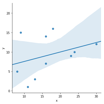
Plotting a univariate regression
import seaborn as sns
sns.lmplot(y='y', x='x', data=df)

If you like the content, please SUBSCRIBE to my channel for the future content.
To get full video tutorial and certificate, please, enroll in the course through this link: https://www.udemy.com/course/python-for-researchers/?referralCode=886CCF5C552567F1C4E7
